TION
Finger photoplethismography
(PPG) is a commonly used technique in medical services. In most
of the cases it is used for measuring the heart rate. A recent
research suggests the possibility to use plethismography for measuring
blood pressure and other indices of peripheral vascular activity
[2,4,14,15,17].
However, it has been pointed out that there may be difficulties
related to wrong data interpretation [3,6].
Nevertheless,
several groups suggest that the plethismographic signal carries
very rich information about cardiovascular regulation, which commonly
is not obtained by using the available methods [1,
13,16].
Thus it seems
to be justified the use of advanced signal analysis techniques
for the study of plethismographic signals.
In this work,
we applied a high-degree polynomial detrendening technique in
combination with a kernel nonparametric method for evaluating
plethismographic signal dynamics.
Our results
indicate that the detrendened plethismographic signal is a very
stable, highly nonlinear signal with a very small stochastic contribution.
Application of the kernel nonparametric estimator revealed that
the purely deterministic nonlinear component corresponds to a
low dimensional limit cycle resembling the original appearance
of the phase portrait from original data. The stochastic component
of this signal, however, is not a white noise. At least an important
contribution of 1/f noise may be detected. Regarding its spectral
properties, the noise component shares some of the properties
of heart rate variability signals reported in literature.
Thus, the application of nonlinear techniques allowed separating
three distinct components of the plethismographic signal:
A slow non-stationary
component probably related to recording artifacts.
A non-linear
deterministic component carrying information about the waveform
features, and corresponding to a limit cycle.
A noise non-stationary
component with 1/f dynamics, suggesting at least partial fractality.
This component seems to share important aspects of the R-R signal
described in literature.
The two last
components may carry important information both, about the cardiovascular
and the autonomic nervous system. Thus, we may expect that the
previously mentioned methodology may open new possibilities both
for research as well as for diagnostic purposes.
MATERIALS
AND METHODS
Subjects
Transmission
plethismography (PG) recordings were obtained from six healthy
volunteers (three female and three males), aged 24-46 years (average
age 32 years). The subjects were seated during examination, with
their hands laid comfortably on the table at the level of the
heart. Recording time was 5 min after a rest period of 10-min.
Room temperature was 25 oC.
PPG Recordings
The transmission
PPG probe of the commercial pulse oxymeter (OXY9800-COMBIOMEQ,
Cuba) consisted of a light emitting diode (LED) of 865 nm and
a PIN photodetector (peak spectral response 865 nm) placed on
different sides of the probe, so that they were attached to the
two contralateral surfaces of the finger.
The PPG probe
was attached to the right hand. The computerized system allowed
to optimally adapting the amplification level for obtaining a
nonsaturated signal. The PPG signal was digitized (75 Hz) and
stored in ASCII format. All the statistical processing was performed
off-line.
Data
analysis.
Signal processing
included:
- Power
spectrum estimation.
- Baseline
correction.
- Correlation,
dimension, estimation.
- Fractal
Dimension estimation.
- Nonlinear
Dynamics identification.
Power
spectrum estimation was performed through the FFT
algorithm applied to the original signal [20]. The power spectrum
was estimated as the square of the absolute value of the FFT.
Linear fit was performed to log-log transformed power spectra
for obtaining an estimate of the fractality index a
Baseline
correction was performed by adjusting the whole
signal to a polynomial of the type:

where St is the plethismografic signal evaluated at
time t; a0,a1,…,ak, are
real constants, corresponding to the model’s coefficients.
The order of the model was set at k=22, since this value better
warranties stationarity of the corrected signal without affecting
the shape of the pulsatile waveforms.
The aim of
this procedure is to correct the signal for nonstationarities,
while preserving the original features of the waveform.
Three experts
independently checked for the preservation of the waveform’s
shape after the detrendening procedure.
Correlation
dimension estimation a Grassberger Procaccia algorithm
[10], was applied to the detrendened signals.
In each case the estimated value was compared with that of a surrogate
signal obtained via inverse FFT analysis with phase randomization,
as described in [10]. Two-dimensional projections
of the reconstructed phase portraits were obtained applying the
Taken’s vector method [8].
Nonlinear
Dynamics identification. Kernel nonparametric analysis
was applied to the trend-corrected signals. In kernel autoregression,
the signal is fitted to a model of the type:

The function nonlinear F is obtained as a weighted average of
the observed points in the phase space, the nearest points bearing
the highest contribution. A detailed description of the method
appears in the references [7-11,
18].
During the
application of the kernel procedure, the following information
was obtained:
- Order of
the autoregressive model (r). It reflects the number of past
values necessary to optimally describe the autoregressive function.

Nonlinear
correlation coefficient expressed as:
- where
Vtot corresponds to the signal’s variance and Vne is the
unexplained variance after applying the model.
- In the
linear case, this expression is equivalent to the linear correlation
coefficient [10].
- Noise free
realization generation (NFR). The noise free realization [9,18]
is obtained via sequential estimation of the function F to previously
estimated data points of the time series. The first points of
the series are set at random. The 100 first points of the NFR
are discarded for assuring the absence of transients in the
NFR.
The phase
portrait reconstructed from the NFR gives information about the
noise free dynamical system.
RESULTS
General features
of the signal.
An original,
untreated recording is shown in fig 1.
Fig 1. Photoplethismographic (PPG) signal obtained from a female
healthy subject (age 30 years). Legend: Abscissas-time, expressed
in 13,33-ms time units. Ordinates- PPG signal amplitude in arbitrary
units.
As appreciable,
significant baseline shifts are present in this signal. It is
possible that this is a consequence of recording difficulties
(fixation fails, subject’s movements, etc), though it is
not possible to exclude some physiological influences. A detailed
look up at the signal shows the presence of quite stable waveforms,
whose appearance is relatively little influenced by baseline shifts.
In the literature,
most of the attention is paid to pulsatile waveforms ([1,13,19]).
It could be
plausible to suppose that this signal is a more or less periodic
component affected by random influences. However, some evidences
may not support this view.
In fig 2 a
log-log plot of the signal’s power spectrum is shown. As
appreciable, a linear component with a negative slope could be
appreciated. The estimated slope from the power spectrum is 1.83,
close to that of fractal Brownian process [12].
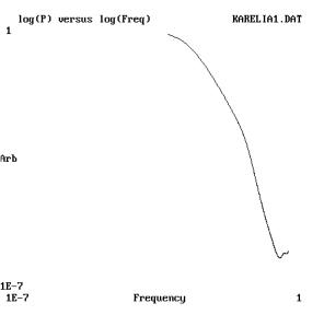
Fig 2. Log-Log
plot of the power spectrum estimated from the recording in 1-a.
Legend: Abscissas, frequency in arbitrary units; Ordinates-Power
spectral density. Notice the presence of a relevant negative slow
linear component. The peak corresponds to the periodic pulsatile
waves.
We applied
a time domain algorithm proposed by Higuchi for the estimation
of the fractal dimension [12]. Higuchi's method
also allows the estimation of the power-spectral slope in log-log
coordinates (a).
The signal’s
dimension was 1.65, which correspond to a fractal process. The
spectral log-log slope (a) estimated by Higuchi’s method
was 1.70, close to that estimated from the power spectrum (1.83,
see above).
Since these
observed features of the original signal may not be explained
by its periodic component, nor by its perturbations with Gaussian
noise, it has sense to try to find out what components may be
responsible for different properties of the PG signal.
Base Line
Correction
Fig 2a. shows
an original signal and the estimated 22-degree-polynomial. As
appreciable, the procedure applied gives a satisfactory estimate
for a time-dependent base line for the original signal.
Fig 2-a. The
recording from fig in 1-a and its time-dependent trend estimated
by fitting to a 22-degree polynomial. Legend: as in fig 1a
After base
line substraction, a detrendened signal was obtained (fig 2b).
Fig 2-b. The
result of subtracting the estimated trend in fig 2a from the signal
in fig 2. This is the trend-corrected component. Legend: as in
fig 2.
Visual appreciation
suggests that the detrendened signal seems to be much more close
to a stationary one than the original signal. This may also be
supported with quantitative data. Fig 2c represents the dependence
of the standard deviation of the signal for both, the original
and the detrendened signal. This dependence for the original signal
is typical for nonstationary time series, included fractal ones
([12,20]).
Fig 2-c. Dependence of the signal’s standard deviation upon
segment’s length for the original trace in fig 2 (upper
line) and for the trend-corrected signal from fig 2b. Legend:
abscissas-time-segment duration in 13.3 ms sampling units. Ordinates:
standard deviation.
At the same
time, the detrendening procedure did not affect the appearance
of the pulse waveforms.
Fig. 3a shows
a 2-dimensional projection of the reconstructed phase portrait.
Fig 3a. S-D
projection of the reconstructed attractor, using the Takens method.
Abscissa St. Ordinates St-10.This picture corresponds to the trend-corrected
signal in fig 2b.
In figure
3b is represented the same phase portrait obtained from another
record taken from the same subject 3 days after. The high stability
of the picture may be suggested from both pictures.
Fig 3b. The
same as in fig 3a, applied to another recording from the same
subject taken three days after. Notice that the difference in
scales accounts for very similar attractor geometry.
The appearance
of this signal could suggest about a low dimensional chaotic dynamics,
very similar to the Rossler attractor.
However, as
shown previously for EEG signals, an alternative explanation may
be that of a limit cycle perturbed by noise [9].
We estimated
the correlation dimension of the detrendened signal. For that
we applied the Grassberger-Procaccia algorithm. The value of correlation
dimension corresponding to the detrendened signal was D=4.694
± 0.662 for an embedding dimension of ED=10. This value
may suggest about a low dimensional chaotic attractor. However,
for the phase surrogate of the detrendened signal this value was
3.64 ± 0.51. Thus correlation dimension value does not
support the hypothesis of a chaotic attractor.
Nonlinear
identification techniques allow to separate deterministic and
stochastic components from a nonlinear stochastic time series.
One of the most powerful methods of nonlinear identification is
the kernel nonparametric autoregressive estimation. However, this
method works satisfactorily only for stationary signals. Thus
the detrendening procedure allowed us to apply a nonlinear identification
method to detrendened data.
Application
of this method to 1000-points segments of the original time series
revealed that the order of the autoregressive model was equal
to 3 in more than 85% of the segments analyzed. The nonlinear
correlation coefficient was higher than 0.99 in all cases, suggesting
the presence of a low-dimensional nonlinear deterministic component
in the detrendened signal.
Fig. 4 shows
a phase portrait obtained from the noise-free realization. The
comparison to figs. 3a and 3b supports the idea of the plethismographic
signal modeled as a limit cycle perturbed by random contributions.
Fig 4. The
same as in fig 3a, applied to a noise-free realization obtained
from applying kernel nonparametric autoregression to the first
1000 points of the trend-corrected recording in fig 2b. Notice
the limit cycle structure of the noise-free attractor.
Though the
generated noise free realization may carry information about the
nonlinear dynamics of pulse wave generation, it obviously may
not account for the fractal-like properties of the original recording.
Properties
of the Residuals
From the application
of the kernel autoregression there still remain the residuals
of the estimation. The residual’s signal may give a good
estimate of the noise component in the model. If we compare the
variance of the noise component to that of the original signal
we may observe that this component seems to be negligible compared
to the original signal or even to the noise free realization (it’s
value never reaches 5% of the variance of the detrendened signal).
However, the
residual’s signal also may contain interesting information.
In particular,
the residuals’ signal (fig 5a) does not seem to be a white
noise signal. Is spectral slope in log-log coordinates is a=1.3
(r=0.73; n=450). Though it is lower than the value of the original
signal this suggests about the presence of fractal components
in the residual’s signal (see fig 5b).
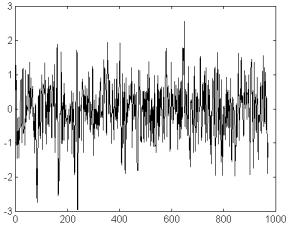
Fig 5a Residuals
after the estimation of the expected values in the recording from
fig 2b. according to the nonlinear nonparametric autoregressive
model. Legend, as for fig 2. Notice the small amplitude of the
signal, compared to fig 2b, or 2a.
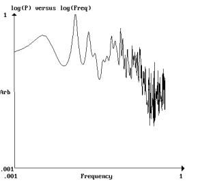
Fig 5b. Log-log
power spectrum of the residual’s signal in fig 5. Legend,
as in fig 2. After discarding the first 15 points on the left
part of the trace, the curve fits to a straight line with a =
0.83 and the linear correlation coefficient r=0.76 (N=450 data
points).
Finally, we
decided to reconstruct a signal composed by the sum of both residuals
and the estimated base line. This signal will carry information
about the original signal with exception of the part corresponding
to a deterministic nonlinear dynamics.
After submitting
this signal to the f Higuchi’s algorithm, the estimated
signal’s fractal dimension was D=1.65, which corresponds
to a value of a=1.71, almost identical to the 1.70 value obtained
from the original data (see above).
Fig. 6 represents
the log-log spectral plot of the baseline-added residual signal.
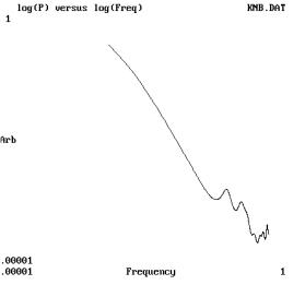
Fig 6- The
log-log power spectrum of the sum of the signal in 5 and the trend
component from fig 2a. Similarity to fig 2 is appreciable.
DISCUSSION
The main results
obtained in this research may be summarized as follows:
The PPG signal
can be represented as a sum of at least three processes, including:
- A low dimensional
nonlinear component with a periodic attractor, which accounts
for the plethismographic signal waveform, commonly studied [13].
- A more
or less regular high-amplitude-baseline signal, which may be,
approximates as a polynomial function of the time. The baseline
is likely to include both artifacts (patient’s movements,
sensor’s fluctuations, etc) and physiological components
(tissue replenishing with blood, respiration, etc. [16]).
- A low-amplitude
random component with fractal-like properties.
The original
signals present not only periodicities due to the presence of
the pulse waves, but also fractal-like properties. The sum of
the baseline and the residual’s signal (after applying a
kernel nonparametric method) may account for the fractal-like
properties of the original signal.
Thus our results
suggest that it is possible to separate the plethismographic signal,
via nonlinear filtering, into components carrying different types
of information.
In our opinion,
our results open new possibilities, and, at the same time, give
birth to new questions.
Thus the fact
that the nonlinear deterministic part of the signal may be modeled
with a nonparametric function of order 3 opens the possibility
to find an analytical model for this component generation. Since
this component is related to arterial compliance and resistance,
as well as other factors contributing to blood volume increase
during systole [16], this may open new possibilities
for research and diagnosis of blood pressure regulation.
It seems difficult
to determine the possible physiological components of the baseline
signal. Though literature data refer to the baseline as inversely
related to the blood volume in the tissue under examination [16],
it is not excluded the contribution of recording artifacts to
this signal. Thus, as described in [1] minor
movements of the arm may change the signal baseline. It seems
reasonable to suppose that physiologically-conditioned factors
contribute to the fractality of the original signal, which could
not be expected from low frequent trends in the signal.
At the same
time, it seems difficult to ignore the physiological implications
of the fractality of the low amplitude residual (noise) signal.
A considerable
experimental material supports the idea of a partially fractal
nature of heart rate variability signals [5,20].
However, the
HRV signal is contained in the electrocardiogram, and, as assumed
also in the plethismographic signal [16].
The signals
analyzed were relatively short in terms of HRV analysis, and lasted
fractions of a minute. However, if we believe in the truly fractality
of a process, it must be present not only at long-range time scale,
but also at microscopic scales [5].
On the other
hand different authors have claimed the fractal nature of ECG
complexes [5]. Thus it would not be surprising
to find a physiologically conditioned fractal component in the
PPG signal.
A major task
remains to identify the physiological bases of these processes.
In literature, several attempts have been made, as for example
those related to interpret the fractal nature of the QRS-complex
in the ECG as emerging from the fractal nature of the Hiss bundle
[5].
Experimental
research by Yamamoto suggested that the HRV fractal component
is not affected by beta blocking, which suggests involvement of
factors different from the autonomic nervous system in this process
[20].
The possible
diagnostic utility of these results also open new perspectives.
Some of these questions are subject of further analysis by our
group.
REFERENCES
1.
Allen J, Murray modeling the relationship between peripheral blood
pressure and blood volume pulses using linear and neural network
system identification techniques. A Physiol Meas 1999 Aug;20(3):287-30.
2. Bruner, J. M. R. (1981). Comparison of direct
and indirect methods of measuring arterial blood pressure. Medical
Instrumentation, 15, 11-12.
3. Escourrou PJ, Delaperche MF, and Visseaux A,
"Reliability of Pulse Oxymetry during Exercise in Pulmonary
Patients", Chest, 1990, 97 (3): 635-8.
4. Frey, W. Butt, Neonatal and pediatric intensive
care: Pulse oxymetry for assessment of pulsus paradoxus: a clinical
study in children, Intensive Care Medicine 24 (1998), 242-246.
5. Goldberger, A.L. Fractal Mechanisms in the
electrophysiology of the heart. IEEE Transactions on Engineering
in Medicine and Biology (11): 47-52, 1992.
6. Gregorini P, Gallina A, and Caporaloni M: Comparison
of One Minute versus Five Minute Sampling Rate of Physiologic
Data. The Internet Journal of Anesthesiology 1997; Vol1N4:
http://www.ispub.com/journals/IJA/Vol1N4/sampling.htm.
7. Haerdle W, Luetkepohl H, Chen R. A review of
nonparametric time series analysis Int Stat Rev. 1997 65 1: 49-72.
8. J. L. Hernández, L. García, Guido
Enzmann, A. García. “La regulación autonómica
del intervalo cardíaco modelada como un sistema no lineal
estocástico con múltiples atractores”. Revista
CENIC. Ciencias Biológicas. Vol. 30, No 3, 1999.
9. J. L. Hernández, P. Valdés and
P. Vila. "Spike and wave activity with a limit cycle perturbed
by noise". NeuroReport, Vol. 13, 1996.
10. Hernández JL, Valdés JL, Biscay
R, Jiménez JC, Valdés P. "EEG predictability.
Adequacy of nonlinear forecasting methods". Int J Biomed
Comput. 38 197-206 (1995).
11. Hernández, J. L., Biscay, R, Jiménez,
JC, Valdés P, Grave de Peralta, R. "Measuring the
dissimilarity between EEG recordings through a non linear dynamical
system approach". Int J. Biomed. Comput. 38, 121-125 (1995).
12. Higuchi Physica D, 1990.
13. Imanaga I, Hara H, Koyanagi S, Tanaka K Correlation
between wave components of the second derivative of plethismogram
and arterial distensibility. Jpn Heart J 1998 Nov;39(6):775-84.
14. Jennings, J. R., Tahmoush, A. J., & Redmond,
D.P. (1980). Non-invasive measurement of peripheral vascular activity.
In I. Martin & P. H. Venables (Eds.), Techniques in Psychophysiology.
John Wiley & Sons, Ltd.: New York.
15. Mineo R, Sharrock NE Pulse oximeter waveforms
from the finger and toe during lumbar epidural anesthesia. Reg
Anesth 1993 Mar-Apr;18(2):106-9.
16. M. Nitzan, A. Babchenko, B. Khanokh. Very
low variability in arterial blood pressure and blood volume pulse.
Med. Biol. Eng. Comput., 1999, 37, 54-58.
17. Rumwell C.,McPharlin M: In Vascular Technology,
an illustrated review for the registry exam. Davies Publishing
Inc., Pasadena, CA, 1996.
18. P. Valdés, J. Bosch, J. C. Jiménez,
N. Trujillo, R. Biscay, F. Morales, J. L. Hernández, T.
Ozaki. The statistical identification of nonlinear brain dynamics:
A progress report. In: “Nonlinear Dynamics and Brain Functioning”.
Pradhan N., Rapp P. E. And Sreenivasan (Eds.), Nova Science Publishing,
1999.
19. M. Wolf Pulse Oxymetry and Medical Infrared
Spectroscopy http://www.biomed.ee.ethz.ch/staff/ibt_members.html
(1998).
20. Yamamoto, Y., Hughson, R.L. Coarse graining
spectral analysis: new method for studying heart rate variability.
Journal of Applied Physiology (71): 1143-1150,1991.